Second-Order Differential Equations
Table of Contents
m to reveal the entire page or ? to show all shortcuts.
We have seen how to solve first-order differential equations of the form
\begin{equation} \frac{d v}{d t} = f(v) \qquad\text{or}\qquad \frac{d x}{d t} = g(x) \label{eq:firstorder} \end{equation}
However, Newton’s equations of motion (in one dimension) are typically second-order
differential equations of the form \[ m \frac{d^2 x}{dt^2} = F(x, v, t) \] where
\(v = dx/dt\) and \(F\) is some function of the position, velocity, and time. We have seen how
we can use Euler’s method to develop an approximate numerical solution to a first-order
equation, where we use the fact that we know the function that computes the derivative,
and we can use small but finite steps to estimate the true solution. We have also seen
that nifty functions like solve_ivp can use higher-order numerical methods to compute
more accurate solutions to first-order equations without having to take really tiny
steps. Wouldn’t it be nice if we could somehow take advantage of these tools to solve
second-order differential equations?
1. Objectives
In this unit you will learn
- How to develop an approximate numerical solution to a second-order differential equation.
- How to compute a smooth solution to the equation over a given temporal range.
- How to generalize to any number of simultaneous first- or second-order differential equations.
- How to test whether a solution makes sense.
2. The Secret
As it turns out, we can leverage all we have learned to handle a second-order equation! The trick is to use twice as many first-order equations. Let’s see how that can work using a particularly simple example. Suppose we wish to solve
\begin{equation} m\ddot{x} = - k x \end{equation}which describes a particle of mass \(m\) subject to a restoring force that grows linearly with displacement from \(x = 0\). (Remember that the dots signify derivatives with respect to time.)
If we use more conventional notation, in which \(\dot{x} = v\) and \(\ddot{x} = \dot{v}\), we could write
\begin{align} \dot{v} &= - \frac{k}{m} x \\ \dot{x} &= v \end{align}each of which is a first-order equation. That is, by introducing as a new variable the first-derivative of position with respect to time (\(v\)), we can break apart the single second-order equation into two coupled first-order equations.
Let’s say that again. To solve a second-order differential equation of the form
\begin{equation} \ddot{x} = f(x, \dot{x}, t) \end{equation}use two dependent variables, \(x\) and \(v\), to write the coupled equations
\begin{equation} \left[\ \begin{array}\ \dot{x} \\ \dot{v} \end{array} \right] = \left[\ \begin{array}\ v \\ f(x, v, t) \end{array} \right] \end{equation}
then we can use Euler’s method—or the better methods of solve_ivp —to solve
simultaneously for \(x(t)\) and \(v(t)\). Recall that the call signature of
solve_ivp is solve_ivp(deriv_func, time_range, initial_values, ...).
Fortunately, the deriv_func can return an array of derivatives, and the
initial_values can be a corresponding array of the initial values of the
coordinates. Let’s see how the example plays out.
# First prepare the notebook by loading the necessary modules

%matplotlib notebook

import numpy as np

import matplotlib.pyplot as plt

from scipy.integrate import solve_ivp
We have to define a function that computes the vector of derivatives at time \(t\) and a vector of the coordinates, \(X = [x, v]\). We can list the coordinates in any order we like, as long as use the same order for the derivatives, \([\dot{x}, \dot{v}]\).
def SHOderivs(t, X, k, m):

  """

  Compute the derivatives of a simple harmonic oscillator of mass m and spring constant k

  where the dependent variable X holds [x, v].

  """

  x, v = X # we use x = X[0] and v = X[1]

  # the derivative dx/dt = v, and

  # the derivative dv/dt = -k/m * x

  # we have to return the derivatives in the same order as the coordinates

  # were delivered in X

  derivs = np.array([v, -k/m * x])

  return derivs
Note again that this function receives the coordinates [x, v] in a list (array)
in the variable X, so it returns the derivates [v, a]. We can now integrate
the differential equation for the time range \(0 \le t \le 1\), starting with
\(x(0) = 1\) and \(v(0) = 0\).
 res = solve_ivp(SHOderivs, [0, 1], [1.0, 0.0],

                 t_eval=np.linspace(0, 1, 21), args=(4, 0.25))

 res


 message: 'The solver successfully reached the end of the integration interval.'

        nfev: 56

        njev: 0

         nlu: 0

         sol: None

  status: 0

 success: True

           t: array([0.  , 0.05, 0.1 , 0.15, 0.2 , 0.25, 0.3 , 0.35, 0.4 , 0.45, 0.5 ,

          0.55, 0.6 , 0.65, 0.7 , 0.75, 0.8 , 0.85, 0.9 , 0.95, 1.  ])

t_events: None

           y: array([[ 1.        ,  0.98006663,  0.92107572,  0.825395  ,  0.6967433 ,

                0.54024223,  0.36225911,  0.16986033, -0.02929309, -0.22738616,

           -0.41646995, -0.58889897, -0.73787313, -0.85727112, -0.94240378,

           -0.9900373 , -0.99845565, -0.96702272, -0.89675673, -0.79050156,

           -0.65289549],

          [ 0.        , -0.79467787, -1.55781879, -2.25895497, -2.86969046,

           -3.36596441, -3.72862823, -3.94317039, -3.99972153, -3.89581286,

           -3.63647339, -3.23315991, -2.7011724 , -2.06107624, -1.33812055,

           -0.56208386,  0.23632515,  1.02504019,  1.77273867,  2.45002813,

                3.0295073 ]])

y_events: None
Looking at the output of solve_ivp, we see that the array returned as y is
now two-dimensional, since our coordinate “vector” consists of X = [x, v]. Let's
make a plot of the solution.
fig, ax = plt.subplots()

t = res.t

x = res.y[0,:]

v = res.y[1,:]

ax.plot(t, x, 'ro', label="$x$")

ax.plot(t, v, 'bo', label="$v$")

ax.legend()

ax.set_xlabel('$t$');
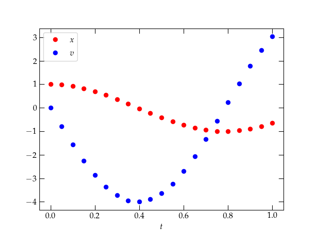
Figure 1: The solution to Eq. (2) provided by solve_ivp.
This plot looks very promising. It looks like the start of an oscillation, which you might expect for a mass suspended from a spring. After all, the differential equation we’re solving is
\begin{equation} \frac{d^2 x}{dt^2} = - \frac{k}{m} x \end{equation}which simplifes to
\begin{equation} \frac{d^2 x}{dt^2} = - 16 x \end{equation}for the particular values of \(k = 4\) and \(m = 1/4\) that we used in our solution. As you can readily verify, the function
\begin{equation} x = \cos(4t) \end{equation}solves this equation. Furthermore, its derivative vanishes at \(t = 0\), as we require. Let’s add this function to the plot to see how the numerical solution is doing.
fig, ax = plt.subplots()

t = res.t

x = res.y[0,:]

ax.plot(t, x, 'ro', label="$x$")

tvals = np.linspace(0, 1, 51)

xvals = np.cos(4 * tvals)

ax.plot(tvals, xvals, 'g-', label=r"$x_{\mathrm{true}}$")

ax.legend()

ax.set_xlabel('$t$')

ax.set_ylabel('$x$');
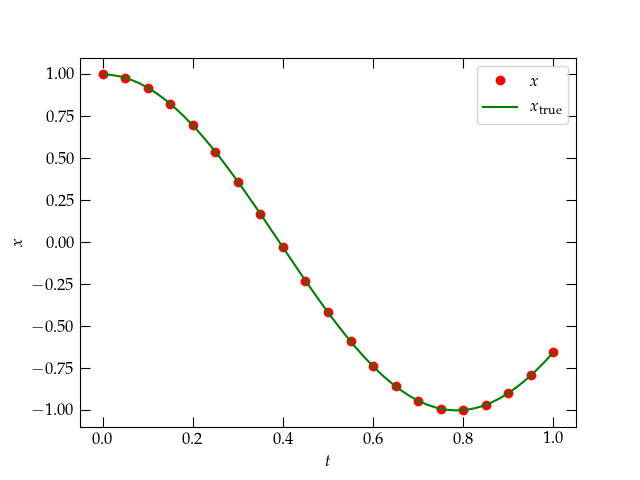
Figure 2: blah
2.1. Exercise
That agreement between the theoretical curve and the numerical solution looks very good, but we
expect that there will be some errors in the numerical solution. Make a plot of the errors for
both \(x\) and \(v\). How small do you have to make rtol to produce an “acceptable” level of error,
in your opinion?
3. Smooth output
So far, we have asked solve_ivp to produce a solution at specific values of
the independent variable \(t\), which we specify by the keyword parameter
t_eval set to a list or array of values. It can be useful, however, not to
have to specify the particular values at the start, but to have solve_ivp
return a smooth function. We can manage this by asking for
dense_output=True. Let’s see how this works.
res = solve_ivp(SHOderivs, [0, 1], [1.0, 0.0], dense_output=True, args=(4, 0.25))

res


          message: 'The solver successfully reached the end of the integration interval.'

                 nfev: 56

                 njev: 0

                  nlu: 0

                  sol: <scipy.integrate._ivp.common.OdeSolution object at 0x137e455e0>

           status: 0

          success: True

                        t: array([0.00000000e+00, 6.24375624e-05, 6.86813187e-04, 6.93056943e-03,

                   6.93681319e-02, 2.63647530e-01, 5.07499921e-01, 7.37486428e-01,

                   9.86950372e-01, 1.00000000e+00])

         t_events: None

                        y: array([[ 1.00000000e+00,  9.99999969e-01,  9.99996226e-01,

                         9.99615762e-01,  9.61750781e-01,  4.93512971e-01,

                        -4.43557322e-01, -9.81750147e-01, -6.91522218e-01,

                        -6.52895491e-01],

                   [ 0.00000000e+00, -9.99000989e-04, -1.09889972e-02,

                        -1.10874908e-01, -1.09570295e+00, -3.47885073e+00,

                        -3.58484295e+00, -7.59559602e-01,  2.88912221e+00,

                         3.02950730e+00]])

         y_events: None
Notice that the output now includes an OdeSolution object in res.sol. We can
use it to evaluate the solution at a point in time within the range we have
simulated as follows:
res.sol(0.5)


array([-0.41646995, -3.63647339])
The solution returns an array (vector) of values of the dependent variables \([x, v]\). Here's how we can use the solution to make a nice smooth plot of the results. We’ll plot the velocity:
tvals = np.linspace(0, 1, 101)

Xvals = res.sol(tvals)

fig, ax = plt.subplots()

ax.plot(tvals, Xvals[1,:], 'r.-', label=r'$v$')

ax.set_xlabel('$t$')

ax.set_ylabel('$v$');
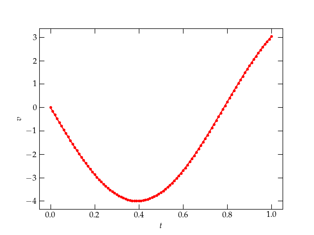
Figure 3: blah
Let’s see what the error in the velocity looks like:
errors = Xvals[1,:] + 4 * np.sin(tvals * 4)

fig, ax = plt.subplots()

ax.plot(tvals, errors, '.')

ax.set_xlabel('$t$')

ax.set_ylabel('Error in $v$');
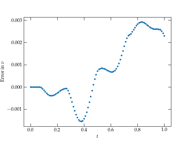
Figure 4: blah
4. Practice
Now, choose a (set of) differential equation(s) to integrate and write a function that takes in a vector of coordinates and returns the derivatives of those coordinates. Suggestions for systems you could use:
- A simple harmonic oscillator: \(\ddot{x} = -\frac{k}{m} x\) for which the analytic solution is \[x(t) = x_0 \cos\omega t + \frac{v_0}{\omega} \sin\omega t\] where \(\omega = \sqrt{k/m}\). Use coordinates \([x, v]\), and the derivatives \([v, -\omega^2 x]\).
- A damped simple harmonic oscillator: \(\ddot{x} = -\frac{k}{m} x - \frac{b}{m} \dot{x}\), which has analytic solution
\[x(t) = \left(x_0 \cos \omega_1 t + \frac{v_0 + \beta x_0}{\omega_1} \sin\omega_1 t\right) e^{-\beta t}\] for \(\beta = 2b/m\), \(\omega_0 = \sqrt{k/m}\), and \(\omega_1 = \sqrt{\omega_0^2 - \beta^2}\). Use coordinates \([x, v]\), and the derivatives \([v, -\omega_0^2 x - \beta v]\) for \(\omega_0 = \sqrt{k/m}\).
- A projectile subject to linear drag:
\[ \ddot{x} = -g - \frac{b}{m} \dot{x} \] which has the solution \[ x(t) = x_0 - v_T\left(t + \frac{e^{-\beta t}}{\beta} \right) + \frac{v_0}{\beta}(1 - e^{-\beta t}) \] where \(\beta = b/m\) and the terminal velocity is \(v_T = m g / b = g / \beta\). Use coordinates \([x, v]\) and the derivatives \([v, -g - \frac{b}{m} v]\).
- A planet subject to the Sun’s gravitational pull, \([r, \dot{r}, \theta,
\dot{\theta}]\), and you figure out the derivatives. Recommendation: use
A.U. for distances and years for times. Hints: \(GM = 4\pi^2\) in these units,
and you can take advantage of the fact that an inverse square force law
produces closed orbits. You might want to use
plt.polar(θ, r)to make polar plots of the trajectories.
Then call solve_ivp with your function and see how well it does. Investigate
how the error depends on the method and/or the tolerances (rtol or
atol). Use a log-log plot for the absolute value of the error.
5. Generalizing to multiple variables
The step to handling more than one variable is now very small. For each second derivative, we use two variables, one for the coordinate and one for its first derivative, to get the coupled equations
\begin{equation} \left[ \begin{array}\ \dot{x}_1 \\ \dot{v}_1 \\ \dot{x}_2 \\ \dot{v}_2 \end{array} \right] = \left[ \begin{array}\ v_1 \\ \ddot{x}_1 = f_1(t, x_1, v_1, x_2, v_2) \\ v_2 \\ \ddot{x}_2 = f_2(t, x_1, v_1, x_2, v_2) \end{array} \right] \end{equation}
Then we pack all these dependent variables in a single array X and supply a
function that computes each one’s derivatives like so:
def bigderivs(t, X, *other_parameters):

  x1, v1, x2, v2 = X # break apart the individual variables, for convenience

  a1 = ...           # compute the acceleration of coordinate 1

  a2 = ...           # compute the acceleration of coordinate 2

  return np.array([v1, a1, v2, a2]) # return the vector of derivatives
The argument *other_parameters is a list of any additional parameters that our
function may require to evaluate the derivatives. When you precede a variable
name with an asterisk, it means that the variable holds a (possibly empty)
list. (When you precede a variable name with a double asterisk, the variable
holds a dictionary of key-value pairs. It’s the way optional keyword arguments
may be passed to a function.)
5.1. Exercise
A conical pendulum is a point mass suspended by a rigid rod that is held fixed at a frictionless pivot. Before we attempt a general solution for arbitrarily large angles with respect to the vertical, we could attempt a solution valid for small angles. Let’s use a cartesian coordinate system with \(z\) pointing up, so the $x$-\(y\) plane is horizontal. For a pendulum of length \(\ell\), it is possible to show that in the case of small displacements from equilibrium, the accelerations in the \(x\) and \(y\) directions are given by
\begin{align} \ddot{x} &= -\frac{g}{\ell} x \\ \ddot{y} &= -\frac{g}{\ell} y \end{align}Write a function that computes the derivatives for such a conical pendulum in the small-amplitude limit and investigate the behavior of the solution for different initial conditions.
- Does your solution produce closed figures in the $x$-\(y\) plane?
- Can you think of a way to check whether energy is conserved? Try ignoring any velocity along the \(z\) axis, as a first approximation, and consider gravitational potential energy and kinetic energy.
- Later we will develop the notion of angular momentum and see that the component of angular momentum parallel to gravity should be conserved for this system. For this system, the angular momentum around the \(z\) axis should be the mass of the bob times the quantity \(x \dot{y} - y \dot{x}\). Is it in fact conserved?