Jupyter Notebooks
Table of Contents
m to reveal the entire page or ? to show all shortcuts.
Jupyter notebooks use a browser to provide an interactive computation and authoring environment that allows one freely to combine text (including LaTeX equations), graphics, computation, and the results of computations in a single window.
An Anaconda installation should already have Jupyter notebook installed and available, but you don't need the full anaconda distribution to use Jupyter notebook.
1 Installation
1.1 Anaconda
If you have anaconda installed you can launch the Anaconda Navigator from which you can launch Jupyter notebook. You can download Anaconda from https://www.anaconda.com/ . According to this note, if you had an Anaconda distribution on a Macintosh and then upgraded to Catalina (10.15), it was likely moved to an unusable location inside a Relocated Items folder somewhere. If this misfortune has befallen you, it appears that the easiest solution is to reinstall Anaconda and be sure to locate the installation somewhere within your home folder.
1.2 Python
If you have a Python installation, and pip is available, you can install everything you need with the following. If you prefer, you can first create a virtual environment for this Python installation so any upgrades or installed libraries don't encounter conflicts:
virtualenv jup              # the standard virtualenv package
# or, if you use the fish shell, as I do
vf jup
pip3 install --upgrade pip  # make sure you have an up-to-date version
pip3 install numpy scipy matplotlib jupyter
These commands install the minimum you need to get going. However, I recommend also installing two more packages:
pip3 install autopep8 ipympl jupyter_contrib_nbextensions
jupyter contrib nbextension install --user
1.3 Configuring extensions
Launch Jupyter notebook from the directory where you would like to load code and save notebooks:
> cd ~/Documents/testing
> jupyter-notebook
A browser window should open and you will see a listing of the files in the current directory. If you installed the nbextensions package, you should also see a menu item called Nbextensions, as illustrated in the figure.
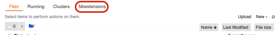
Figure 1: The top of a Jupyter notebook window showing the Nbextensions menu item
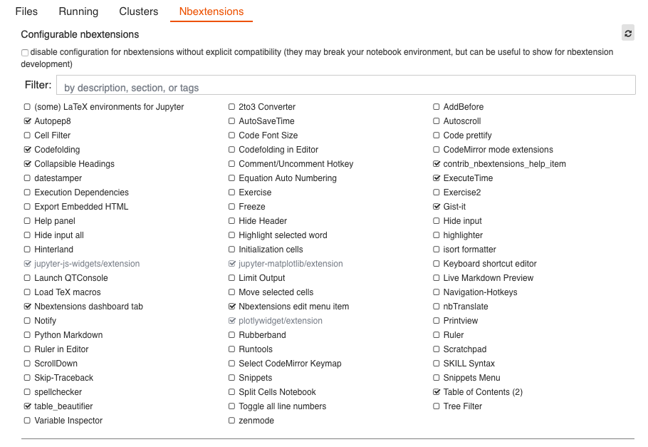
Clicking on the Nbextensions menu will allow you to load extensions as desired. I recommend several, including
- Autopep8
- Codefolding
- Collapsible Headings
ExecuteTime
1.4 Possible configuration additions
By default, Jupyter notebooks have a maximum column width that works great
for managing readable text, but can be too narrow if you have lots of screen
real estate and want to use it in constructing (interactive) plots. You can
adjust the default properties by creating a file to hold custom.css
definitions. On UNIX systems, the custom configuration is stored at
~/.jupyter/custom/custom.css. Your mileage on Windows may differ, so check
the Jupyter documentation. Make sure that both the ~/.jupyter/ and
~/.jupyter/custom/ directories exists, then use your favorite text editor
to generate the following content:
$emacs ~/.jupyter/custom/custom.css

.container {
  width: 90% !important;
  margin-left: 40px;
  margin-right: 40px;
}
2 Getting Started
Launch jupyter notebook (either use Anaconda Navigator or jupyter notebook
from the command line on a UNIX system) to display a directory page.
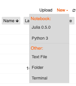
Figure 3: Creating a new Jupyter notebook. Select Python 3.
In the first cell of the new notebook, enter
%matplotlib notebook
import matplotlib.pyplot as plt
import numpy as np
import scipy as sp
and press Shift-Return (Shift-Enter) to submit these instructions to the jupyter kernel.
The first line is “magic” code to allow graphical output from matplotlib to be inserted directly into the notebook. The rest of the lines just load some standard modules with their common abbreviations.
To illustrate what the %matplotlib magic means, enter the following code in the second cell and press shift-Enter.
frequency = 15 # Hz
t_vals = np.arange(0, 1.0, 0.001) # create an array of time values
x_vals = np.sin(2 * np.pi * frequency * t_vals)
plt.plot(t_vals, x_vals, "r-")
plt.xlabel("Time (s)")
plt.ylabel("Amplitude")
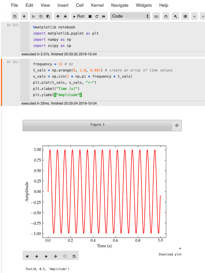
Figure 4: Sample graph in a notebook
3 Configuring MatPlotLib defaults
I dislike matplotlib's defaults. Although it is possible to customize each plot,
it is convenient to put common changes in a preferences file. A copy of the
format file is located in site-packages/motplotlib/mpl-data/matplotlibrc. Save
a copy of this file at ~/.config/matplotlib/matplotlibrc on a unix/linux
system or in $HOME/.matplotlib/matplotlibrc on other systems.
This file has all sorts of options, all of them commented out with leading hash tags. Uncomment the lines you wish to modify and set appropriate values. On my system, I have set the following lines:
saeta@Saeta-MBP16~/.c/matplotlib> grep "^[^ #]" matplotlibrc
backend             : macosx
font.family         : serif # sans-serif
font.size           : 12.0 # 10.0
font.serif          : Utopia, DejaVu Serif, Bitstream Vera Serif, ...
text.usetex         : True # False  ## use latex for all text handling.
xtick.top           : True # False  ## draw ticks on the top side
xtick.direction     : in   ## direction: in, out, or inout
ytick.right         : True ## draw ticks on the right side
ytick.direction     : in   ## direction: in, out, or inout
savefig.format      : pdf  ## png, ps, pdf, svg
savefig.transparent : True ## setting that controls whether figures are saved with a
						   ## transparent background by default
3.1 Using LaTeX in matplotlib labels
If you set text.usetex: True in the configuration file, you can take full
advantage of TeX formatting in labels and annotations. However, beware that
certain characters that have special meaning in TeX, such as the underscore, may
cause labels to throw TeX errors unless they are in math mode. In such cases,
you can explicitly add the keyword argument usetex=False in the command that
produces the text.